If you want to lock cells in Excel, you should protect the worksheet first to get an effect on a particular cell. You cannot effectively lock cells directly without protected the entire worksheet. This means that cells are ready to be locked when you protect the workbook or worksheet. Locking cells or hiding formulas have no effect until you protect the worksheet. In this article, you will get to know how to lock cells in Excel.
How to lock cells in Excel
Follow these below steps to lock cells in the Excel worksheet
- First of all, select the cells that you want to lock.
- Go to the Home tab, and then to the alignment group, now click the small arrow to open the popup window for formatting cells.
- Go to the Protection tab, and select the Locked check box, and then click OK to close the popup.

You can also perform the above action by selecting cells (blank cells or cells having value), and then right-click the mouse and select “Format Cells”.

How to protect a sheet in Excel
Since the default settings in Excel, all cells are locked already.
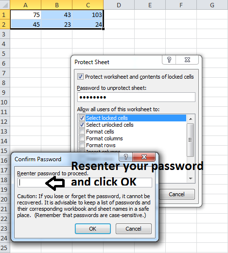
So, when you share an Excel file with someone, you may want to protect a worksheet so that other users cannot be able to do changes in the same worksheet. To protect a worksheet, right-click on the “Worksheet Tab”, and then select “Protect Sheet”.

In the next step, you need to enter the password. Also, you need to check the actions that you want to allow users of your worksheet to perform. Click “OK” after re-entering the password.


That’s it! Your worksheet is protected now. To unprotect a worksheet, right-click on the worksheet tab and click Unprotect Sheet. You will be asked for the password to enter, enter the same password that you just set to unprotect the worksheet.
Leave a Reply